RSeQC
RustQC reimplements eight tools from the RSeQC package (including TIN). Each tool produces output files that match the format and content of the original Python implementation, plus native PNG and SVG plots generated directly — no R scripts required.
All RSeQC tools run automatically as part of the rustqc rna command and use
the input filename stem as a prefix for output files. Output files are organized
into per-tool subdirectories under rseqc/. For example,
rustqc rna sample.bam --gtf genes.gtf -o results/ produces
RSeQC output files like results/rseqc/bam_stat/sample.bam_stat.txt.
Use --flat-output to write all files directly to the output directory instead
of the nested rseqc/<tool>/ subdirectories.
bam_stat
Section titled “bam_stat”Basic alignment statistics from a single-pass BAM scan.
| File | Description |
|---|---|
{stem}.bam_stat.txt | Formatted text report with total records, QC failures, duplicates, mapping quality distribution, splice reads, proper pairs, and more |
The output format matches bam_stat.py exactly, including the same section
headings and number formatting. Key metrics include:
- Total records, QC-failed, duplicates, non-primary, unmapped
- Unique and multi-mapped read counts at the configured MAPQ cutoff
- Read 1 / Read 2 counts, forward/reverse strand counts
- Splice / non-splice read counts
- Proper pair and paired-on-different-chromosome counts
- MAPQ distribution histogram
All values are identical between RSeQC and RustQC on both datasets.
Small dataset
| Metric | RSeQC | RustQC |
|---|---|---|
| Total records | 52,839 | 52,839 |
| QC failed | 0 | 0 |
| Duplicates | 6,097 | 6,097 |
| Non-primary | 3,266 | 3,266 |
| Unmapped | 0 | 0 |
| mapq < cutoff | 1,742 | 1,742 |
| Unique reads | 41,734 | 41,734 |
| Read 1 / Read 2 | 20,871 / 20,863 | 20,871 / 20,863 |
| Sense / Antisense | 20,869 / 20,865 | 20,869 / 20,865 |
| Non-splice / Splice | 22,214 / 19,520 | 22,214 / 19,520 |
| Properly paired | 41,722 | 41,722 |
Large dataset
| Metric | RSeQC | RustQC |
|---|---|---|
| Total records | 201,605,452 | 201,605,452 |
| QC failed | 0 | 0 |
| Duplicates | 132,703,364 | 132,703,364 |
| Non-primary | 15,316,166 | 15,316,166 |
| Unmapped | 12,490,977 | 12,490,977 |
| mapq < cutoff | 2,036,975 | 2,036,975 |
| Unique reads | 39,057,970 | 39,057,970 |
| Read 1 / Read 2 | 19,525,894 / 19,532,076 | 19,525,894 / 19,532,076 |
| Sense / Antisense | 19,529,185 / 19,528,785 | 19,529,185 / 19,528,785 |
| Non-splice / Splice | 27,689,719 / 11,368,251 | 27,689,719 / 11,368,251 |
| Properly paired | 39,030,552 | 39,030,552 |
infer_experiment
Section titled “infer_experiment”Library strandedness inference by sampling reads overlapping gene models.
| File | Description |
|---|---|
{stem}.infer_experiment.txt | Strandedness fractions: failed-to-determine, and the two strand protocols |
The output reports the fraction of reads consistent with each strand protocol:
- Fraction failed to determine — reads that could not be assigned to either protocol
- Fraction “1++,1—,2+-,2-+” (forward stranded) — reads consistent with the same-strand protocol
- Fraction “1+-,1-+,2++,2—” (reverse stranded) — reads consistent with the opposite-strand protocol
For paired-end data, the labels are PairEnd with 1++,1--,2+-,2-+ and
1+-,1-+,2++,2--. For single-end: SingleEnd with ++,-- and +-,-+.
Interpreting results:
- Both fractions near 50% = unstranded library
- First fraction near 100% = forward stranded (e.g., Ligation protocol)
- Second fraction near 100% = reverse stranded (e.g., dUTP protocol, most common)
Strandedness mismatch warning:
RustQC automatically compares the infer_experiment results against the
--stranded flag you specified. If they disagree, a warning is printed
at the end of the run suggesting the correct value:

Small dataset - Identical
| Metric | RSeQC | RustQC |
|---|---|---|
| Failed to determine | 0.0775 | 0.0775 |
| Fraction sense (1++,1—,2+-,2-+) | 0.0051 | 0.0051 |
| Fraction antisense (1+-,1-+,2++,2—) | 0.9174 | 0.9174 |
Large dataset - Minor difference (sampling)
| Metric | RSeQC | RustQC |
|---|---|---|
| Failed to determine | 0.0670 | 0.1052 |
| Fraction sense (1++,1—,2+-,2-+) | 0.0117 | 0.0185 |
| Fraction antisense (1+-,1-+,2++,2—) | 0.9213 | 0.8763 |
The difference is caused by a read-sampling mismatch: the upstream
infer_experiment.py defaults to sampling only 200,000 reads. On a 186M-read BAM,
this early-file subsample draws predominantly from the first few chromosomes, which
underrepresents loci where transcripts on both strands overlap, causing the
“failed-to-determine” fraction to appear lower than it truly is. RustQC processes
all reads, giving a more representative estimate.
Both tools correctly identify the library as strongly reverse-stranded (antisense ~88-92%), so the practical interpretation is identical.
read_duplication
Section titled “read_duplication”Position-based and sequence-based duplication rate histograms.
| File | Description |
|---|---|
{stem}.pos.DupRate.xls | Position-based duplication histogram (TSV: Occurrence, UniqReadNumber, ReadNumber) |
{stem}.seq.DupRate.xls | Sequence-based duplication histogram (TSV: Occurrence, UniqReadNumber, ReadNumber) |
{stem}.DupRate_plot.r | R script for generating duplication rate plots (matching RSeQC format) |
{stem}.DupRate_plot.png | Duplication rate plot (PNG) |
{stem}.DupRate_plot.svg | Duplication rate plot (SVG) |
Each TSV file is a tab-separated table where each row represents a duplication level (number of times a read was seen). The columns are:
- Occurrence — the duplication count (1 = unique, 2 = seen twice, etc.)
- UniqReadNumber — number of unique read groups at this duplication level
- ReadNumber — total reads consumed (Occurrence x UniqReadNumber)
Position-based deduplication groups reads by alignment position (chromosome, start, CIGAR-derived exon blocks). Sequence-based deduplication groups reads by the actual read sequence.
The duplication rate plot shows two curves: mapping-based (blue, x markers) and sequence-based (red, dot markers) duplication. The x-axis shows the occurrence count (capped at 500) and the y-axis shows the number of reads at each duplication level. Most reads should appear at low occurrence counts; a long tail indicates high duplication.
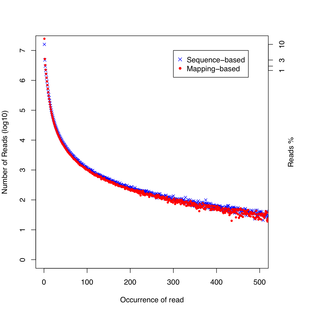
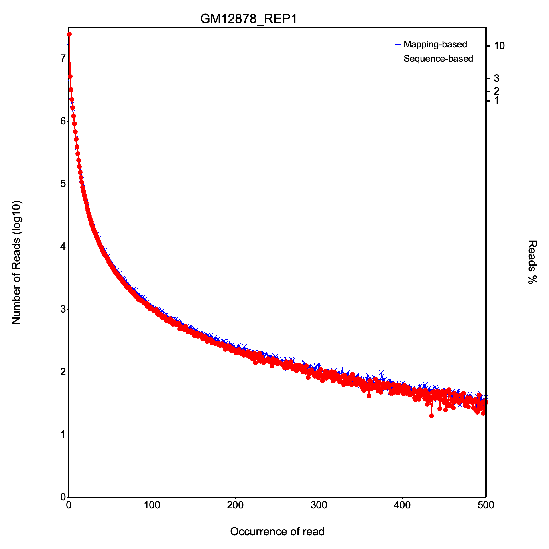
All values are identical on both datasets.
Small dataset (first few duplication levels)
| Level | Seq-based (unique reads) | Pos-based (unique reads) |
|---|---|---|
| 1x | 37,943 | 33,183 |
| 2x | 1,844 | 2,984 |
| 3x | 492 | 693 |
| 4x | 200 | 289 |
Large dataset (first few duplication levels)
| Level | Seq-based (unique reads) | Pos-based (unique reads) |
|---|---|---|
| 1x | 24,661,232 | 15,958,022 |
| 2x | 5,199,146 | 4,781,421 |
| 3x | 3,211,713 | 2,988,951 |
read_distribution
Section titled “read_distribution”Classification of reads across genomic feature types.
| File | Description |
|---|---|
{stem}.read_distribution.txt | Tabular report with total reads, total tags, and per-region breakdown |
The output includes:
- Total Reads and Total Tags (CIGAR M-block midpoints)
- A table of genomic regions with columns: Group, Total_bases, Tag_count, Tags/Kb
- Regions: CDS_Exons, 5’UTR_Exons, 3’UTR_Exons, Introns, TSS_up_1kb, TSS_up_5kb, TSS_up_10kb, TES_down_1kb, TES_down_5kb, TES_down_10kb
- Tags assigned to each region (with priority: CDS > UTR > Intron > Intergenic)
All values are identical on both datasets.
Small dataset
| Feature | Total tags | Tags/Kb |
|---|---|---|
| CDS Exons | 56,186 | - |
| 5’ UTR Exons | 1,226 | - |
| 3’ UTR Exons | 7,495 | - |
| Introns | 2,905 | - |
| Other intergenic | 526 | - |
Total reads: 43,476 | Total tags: 68,660 | Total assigned: 68,134
Large dataset
| Feature | Total tags | Tags/Kb |
|---|---|---|
| CDS Exons | 40,028,987 | 401.24 |
| 5’ UTR Exons | 572,203 | 104.93 |
| 3’ UTR Exons | 5,549,140 | 206.28 |
| Introns | 7,332,516 | 4.87 |
Total reads: 41,094,945 | Total tags: 55,001,331 | Total assigned: 54,113,746
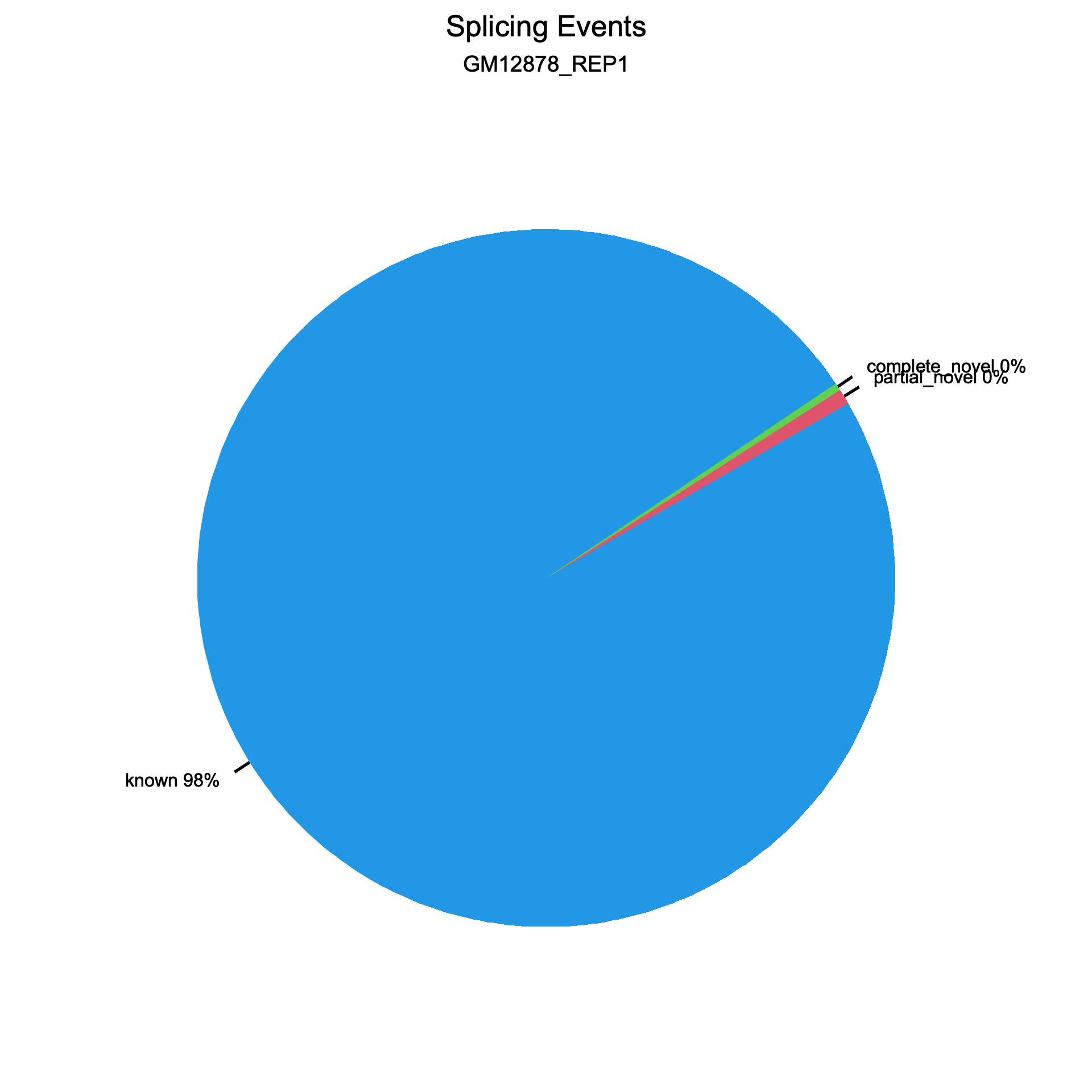
junction_annotation
Section titled “junction_annotation”Splice junction classification against a reference gene model.
| File | Description |
|---|---|
{stem}.junction.xls | TSV with all observed junctions: chrom, intron_start(0-based), intron_end(1-based), read_count, annotation_status |
{stem}.junction.bed | BED12 file with color-coded junctions (red = known, green = partial novel, blue = complete novel) |
{stem}.junction_plot.r | R script for generating splice event and junction pie charts |
{stem}.splice_events.png | Splice events pie chart (PNG) |
{stem}.splice_events.svg | Splice events pie chart (SVG) |
{stem}.splice_junction.png | Splice junctions pie chart (PNG) |
{stem}.splice_junction.svg | Splice junctions pie chart (SVG) |
{stem}.junction_annotation.txt | Summary: total/known/partial novel/complete novel event and junction counts |
Junctions are classified by comparing splice sites (CIGAR N-operations) against the reference gene model:
- Known (Annotated) — both donor and acceptor sites match known introns
- Partial novel — one splice site matches, the other is novel
- Complete novel — neither splice site matches any known intron
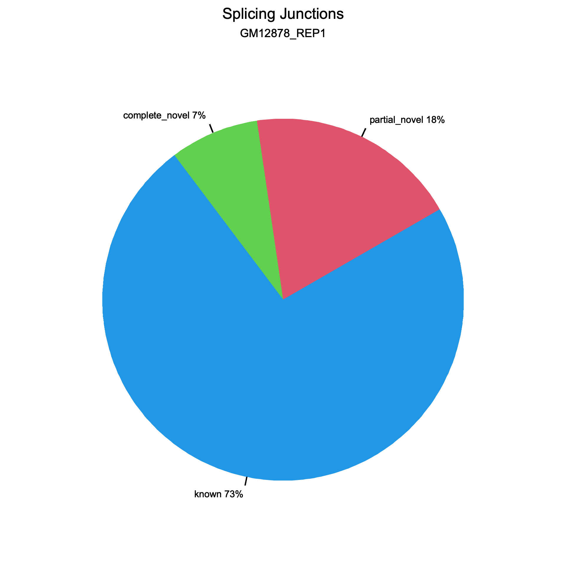
Two pie charts are generated, one for splice events (reads) and one for splice junctions (unique splice sites). Each chart shows the proportion of known (blue), partial novel (red), and complete novel (green) splicing.
Splice events
Section titled “Splice events”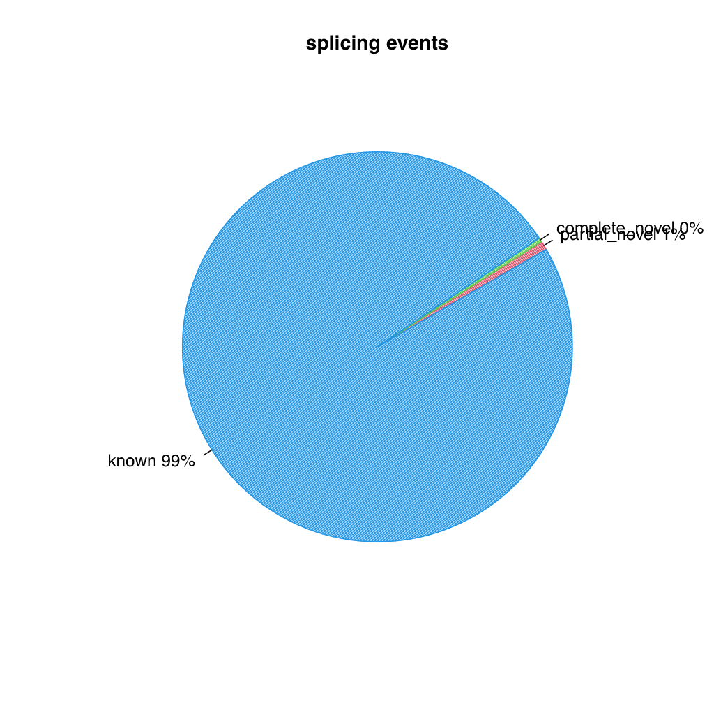
Splice junctions
Section titled “Splice junctions”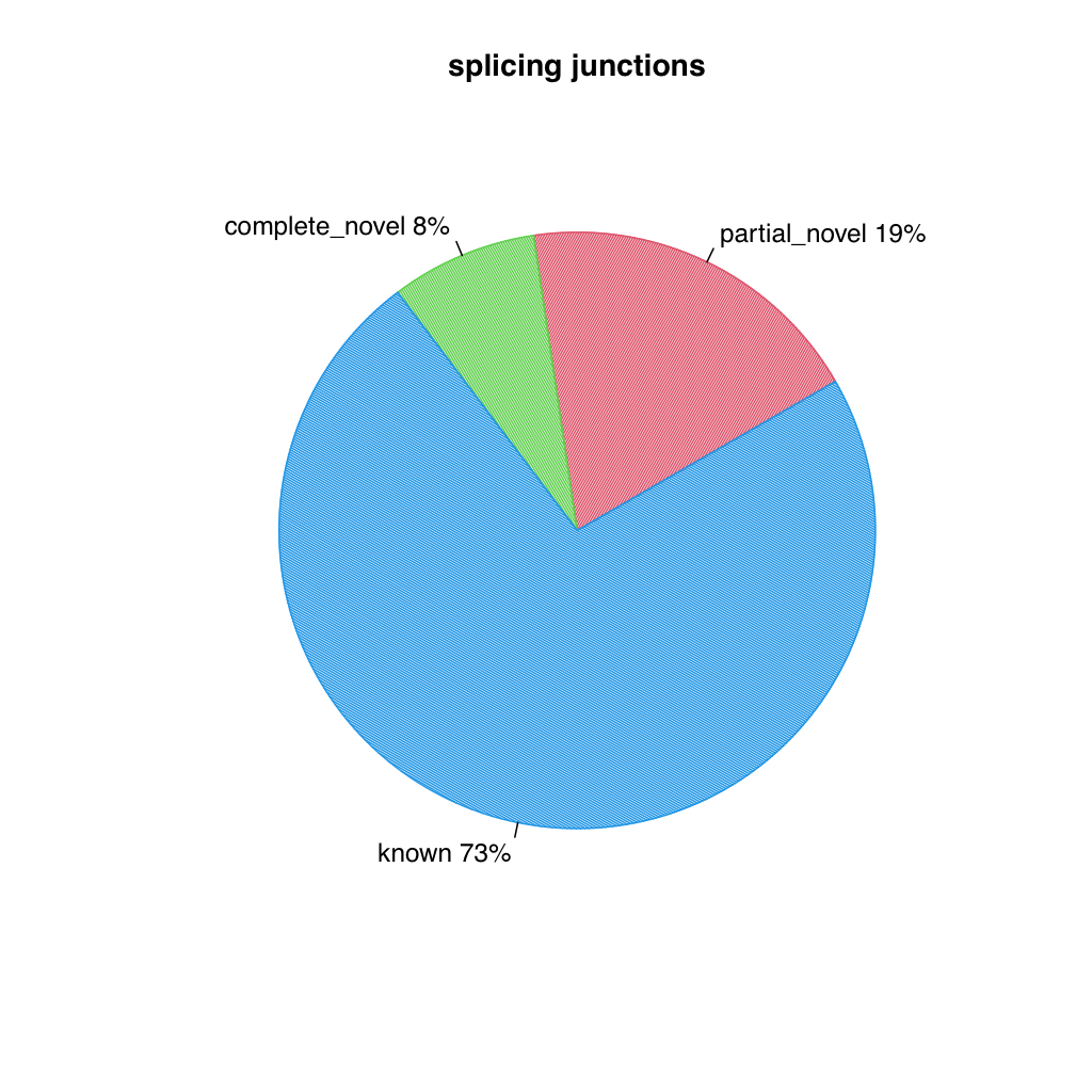
All values are identical on both datasets.
Small dataset
| Metric | RSeQC | RustQC |
|---|---|---|
| Splice events | ||
| Total events | 23,448 | 23,448 |
| Known | 22,625 (96.49%) | 22,625 (96.49%) |
| Partial novel | 166 (0.71%) | 166 (0.71%) |
| Novel | 654 (2.79%) | 654 (2.79%) |
| Splice junctions | ||
| Total junctions | 3,261 | 3,261 |
| Known | 2,982 (91.44%) | 2,982 (91.44%) |
| Partial novel | 88 (2.70%) | 88 (2.70%) |
| Novel | 191 (5.86%) | 191 (5.86%) |
Large dataset
| Metric | RSeQC | RustQC |
|---|---|---|
| Splice events | ||
| Total events | 12,294,654 | 12,294,654 |
| Known | 12,155,894 | 12,155,894 |
| Partial novel | 91,594 | 91,594 |
| Novel | 41,082 | 41,082 |
| Splice junctions | ||
| Total junctions | 239,792 | 239,792 |
| Known | 175,159 | 175,159 |
| Partial novel | 45,554 | 45,554 |
| Novel | 19,079 | 19,079 |
The data files and R plotting scripts match upstream RSeQC output.
junction_saturation
Section titled “junction_saturation”Splice junction discovery rate at increasing sequencing depths.
| File | Description |
|---|---|
{stem}.junctionSaturation_plot.r | R script for saturation curve plots |
{stem}.junctionSaturation_plot.png | Junction saturation plot (PNG) |
{stem}.junctionSaturation_plot.svg | Junction saturation plot (SVG) |
{stem}.junctionSaturation_summary.txt | TSV: percent_of_reads, known_junctions, novel_junctions, all_junctions |
The tool subsamples reads at configurable percentages (default: 5%, 10%, …, 100%) and counts how many unique known and novel junctions are detected at each level. This reveals whether sequencing depth is sufficient for full junction detection. A saturated library will show a plateau in the curve; an unsaturated library will show continuing growth.
The junction saturation plot shows three lines: all junctions (blue), known junctions (red), and novel junctions (green). The x-axis is the percentage of total reads used and the y-axis is the number of splice junctions detected (in thousands). A plateau in the curves indicates saturation.
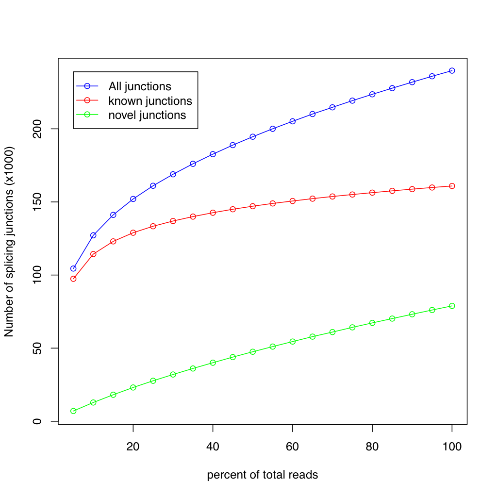
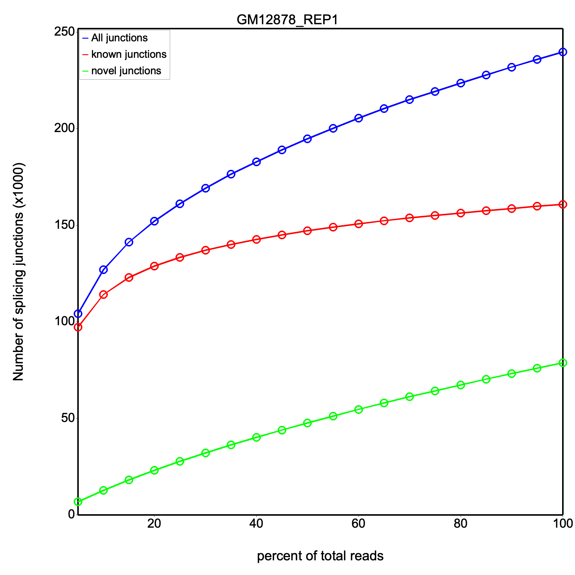
Results are identical between RSeQC and RustQC at full sampling depth on both datasets.
At 100% sampling depth:
Small dataset
| Metric | RSeQC | RustQC |
|---|---|---|
| All junctions | 3,261 | 3,261 |
| Known junctions | 2,944 | 2,944 |
| Novel junctions | 317 | 317 |
Large dataset
| Metric | RSeQC | RustQC |
|---|---|---|
| All junctions | 239,792 | 239,792 |
| Known junctions | 160,896 | 160,896 |
| Novel junctions | 78,896 | 78,896 |
Intermediate sampling percentages show minor stochastic variation from random subsampling, as expected.
inner_distance
Section titled “inner_distance”Fragment inner distance for paired-end RNA-seq libraries.
| File | Description |
|---|---|
{stem}.inner_distance.txt | Per-pair detail: readpair_name, inner_distance, classification |
{stem}.inner_distance_freq.txt | Histogram: lower_bound, upper_bound, count |
{stem}.inner_distance_plot.r | R script for histogram and density plot |
{stem}.inner_distance_plot.png | Inner distance histogram with density overlay (PNG) |
{stem}.inner_distance_plot.svg | Inner distance histogram with density overlay (SVG) |
{stem}.inner_distance_summary.txt | Summary counts by pair classification |
The inner distance is defined as the gap between the end of read 1 and the start of read 2 on the mRNA transcript. Negative values indicate read overlap. Pairs are classified as:
- sameTranscript=Yes, sameExon=Yes — both reads on the same exon
- sameTranscript=Yes, sameExon=No — reads on the same transcript, different exons (distance calculated on mRNA)
- sameTranscript=No — reads on different transcripts or no transcript overlap
- readPairOverlap — reads overlap each other
- nonExonic — one or both reads not on exons
- sameChrom=No — reads on different chromosomes
- unknownChromosome — chromosome not in the gene model
The histogram bins are configurable via --inner-distance-lower-bound,
--inner-distance-upper-bound, and --inner-distance-step (defaults: -250 to 250, step 5).
The inner distance plot is a histogram showing the distribution of fragment inner distances, with a Gaussian density curve (red) overlaid. The title displays the mean and standard deviation. The distribution should be approximately normal for a well-prepared library.
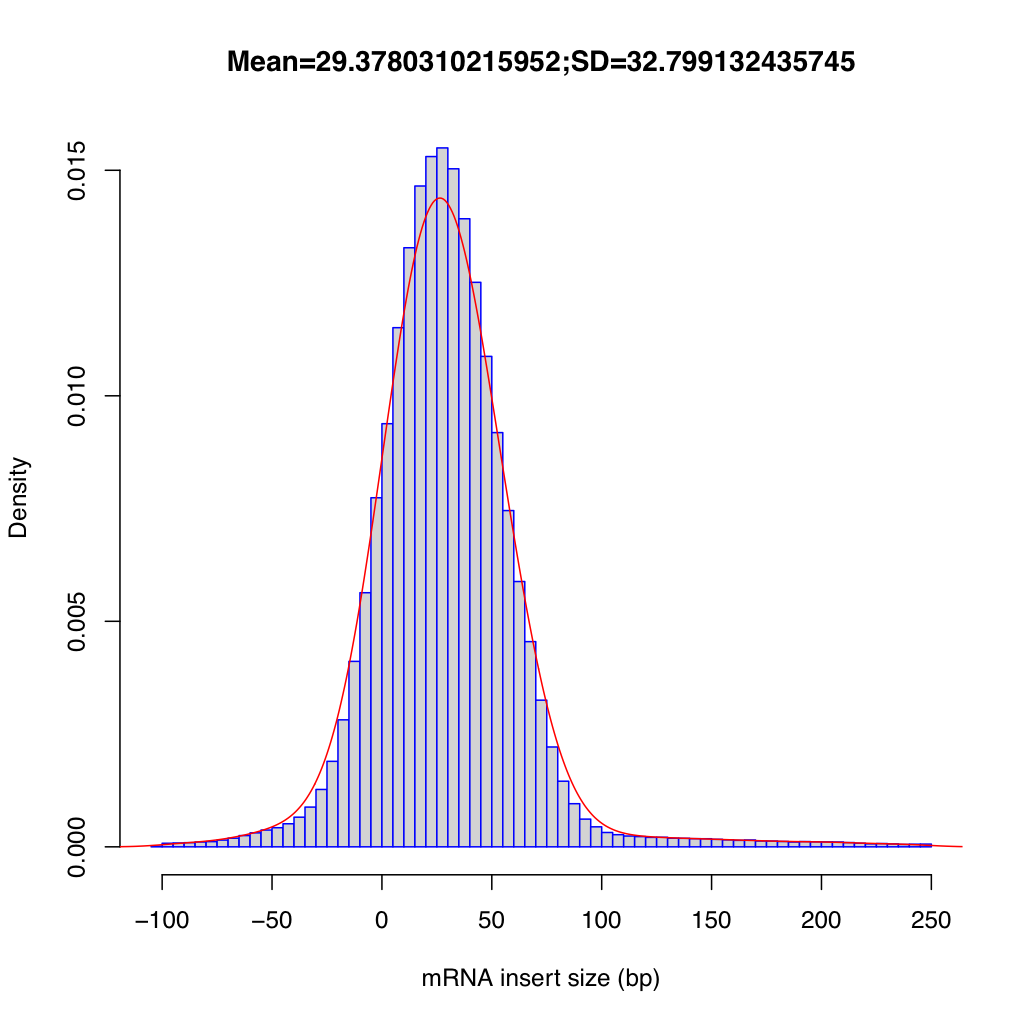
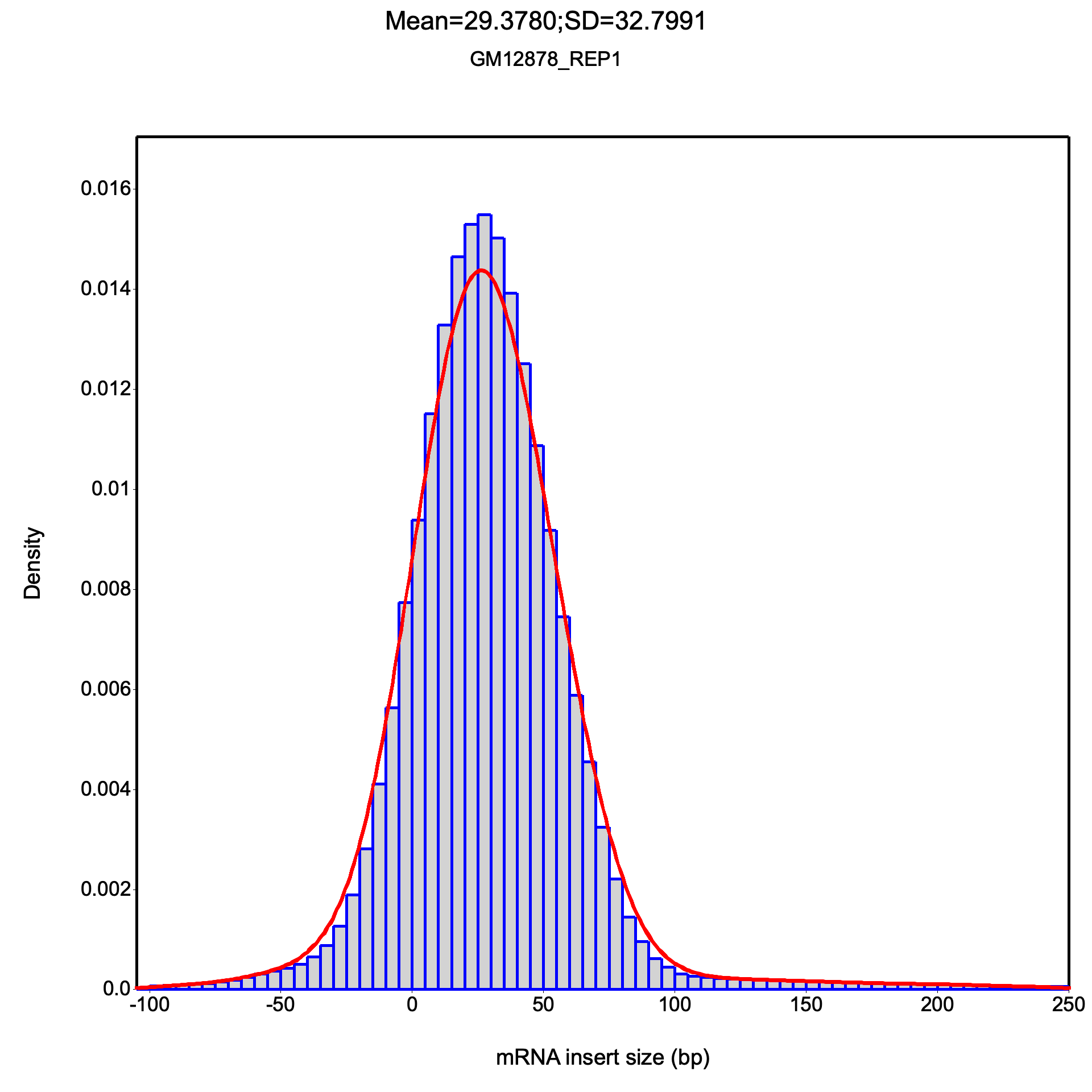
All frequency values are identical on both datasets.
Large dataset summary: mean = 29.378, median = 27.5, std dev = 32.799
The R plotting script (inner_distance_plot.r) matches upstream format exactly.
TIN (Transcript Integrity Number)
Section titled “TIN (Transcript Integrity Number)”TIN (Transcript Integrity Number) measures the uniformity of read coverage across a transcript. A TIN score of 100 means perfectly uniform coverage; lower scores indicate degradation or bias. TIN is computed using Shannon entropy of read-start coverage at sampled positions along each transcript’s exonic regions.
RustQC reimplements RSeQC’s tin.py,
computing TIN scores automatically as part of rustqc rna in the same
single-pass BAM scan as all other analyses.
TIN is particularly useful for:
- Detecting RNA degradation: degraded samples show low TIN scores across most transcripts
- Sample QC: median TIN provides a single-number summary of RNA integrity, complementing RIN (RNA Integrity Number) from Bioanalyzer/TapeStation
- Identifying problematic samples: samples with unusually low median TIN should be flagged for potential exclusion
| File | Description |
|---|---|
{stem}.tin.xls | Per-gene TIN scores (TSV: geneID, chrom, tx_start, tx_end, TIN) |
{stem}.summary.txt | Summary statistics: mean, median, and standard deviation of TIN scores |
TIN scores file
Section titled “TIN scores file”The {stem}.tin.xls file is a tab-separated file with one row per transcript (gene):
| Column | Description |
|---|---|
geneID | Gene identifier from the annotation |
chrom | Chromosome |
tx_start | Transcript start position |
tx_end | Transcript end position |
TIN | Transcript Integrity Number (0-100) |
Transcripts below the minimum coverage threshold are excluded from the output. TIN values are formatted to 2 decimal places.
Summary file
Section titled “Summary file”The {stem}.summary.txt file is a single-row tab-separated summary:
| Column | Description |
|---|---|
Bam_file | Path to the input BAM file |
TIN(mean) | Mean TIN across all transcripts |
TIN(median) | Median TIN |
TIN(stdev) | Standard deviation of TIN |
Interpreting TIN scores
Section titled “Interpreting TIN scores”| Median TIN | Interpretation |
|---|---|
| > 70 | Good RNA integrity |
| 50-70 | Moderate degradation |
| < 50 | Significant degradation — consider excluding |
| < 30 | Severe degradation |
A bimodal distribution of per-transcript TIN scores (some very high, some very low) can indicate selective degradation of certain transcript classes rather than global degradation.
Configuration
Section titled “Configuration”TIN parameters (sample_size, min_coverage) can be set in the YAML config file.
See the Configuration page for details.
TIN uses the shared --mapq / -q flag for mapping quality filtering.
Performance
Section titled “Performance”The upstream tin.py tool processes each transcript independently and scales
poorly with BAM size. On large production datasets (e.g., ~186M reads), tin.py
can take over 9 hours and may fail to complete within typical pipeline time limits.
RustQC computes TIN scores as part of its single-pass BAM scan, completing all
analyses combined in under 15 minutes.
Compatibility
Section titled “Compatibility”RustQC’s TIN output uses the same file format and column names as RSeQC’s
tin.py. TIN scores are computed using the same Shannon entropy formula.
Small dataset - Identical
| Metric | RSeQC | RustQC |
|---|---|---|
| TIN mean | 52.7514 | 52.7514 |
| TIN median | 55.5830 | 55.5830 |
| TIN std dev | 22.5333 | 22.5333 |
Large dataset - Both tools completed
The upstream tin.py took 9h 45m to complete on the large dataset.
RustQC completes TIN analysis as part of its single-pass BAM processing
in under 15 minutes total (inclusive of all other analyses).
| Metric | RSeQC | RustQC |
|---|---|---|
| TIN mean | 70.193 | 70.208 |
| TIN median | 77.980 | 78.007 |
| TIN std dev | 23.588 | 23.597 |
Summary-level TIN statistics are near-identical. Per-transcript TIN values show larger differences due to the coverage counting approach described above.
RustQC produces gene-level TIN scores (one row per gene, using the longest
transcript as representative), while RSeQC’s tin.py produces transcript-level
scores. Both formats are compatible with MultiQC.
Compatibility with RSeQC
Section titled “Compatibility with RSeQC”All output files are designed to be drop-in replacements for the corresponding RSeQC Python tool output. File formats, column names, and numeric precision match the Python originals to facilitate migration from RSeQC to RustQC without downstream pipeline changes.
RustQC also generates the R scripts that RSeQC produces (for junction_annotation, junction_saturation, inner_distance, and read_duplication), maintaining full compatibility. However, unlike RSeQC, RustQC generates the plots directly as PNG and SVG files — there is no need to run the R scripts separately.